pulse code modulation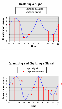

What is PCM?
PCM is a method of converting an analog into digital signals. Information in an analog form cannot be processed by digital computers so it's necessary to convert them into digital form. PCM is a term which was formed during the development of digital audio transmission standards. Digital data can be transported robustly over long distances unlike the analog data and can be interleaved with other digital data so various combinations of transmission channels can be used. In the text which follows this term will apply to encoding technique which means digitalization of analog information in general.

PCM doesn`t mean any specific kind of compression, it only implies PAM (pulse amplitude modulation) - quantization by amplitude and quantization by time which means digitalization of the analog signal. The range of values which the signal can achieve (quantization range) is divided into segments, each segment has a segment representative of the quantization level which lies in the middle of the segment. To every quantization segment (and quantization level) one and unique code word (stream of bits) is assigned. The value that a signal has in certain time is called a sample. The process of taking samples is called quantization by time. After quantization by time, it is necessary to conduct quantization by amplitude. Quantization by amplitude means that according to the amplitude of sample one quantization segment is chosen (every quantization segment contains an interval of amplitudes) and then record segments code word.

To conclude, PCM encoded signal is nothing more than stream of bits
The first example of PCM encoding
In this example the signal is quantized in 11 time points using 8 quantization segments. All the values that fall into a specific segment are approximated with the corresponding quantization level which lies in the middle of a segment. The levels are encoded using this table:
LevelCode word00001001201030114100510161107111Table1. Quantization levels with belonging code words

The first chart shows the process of signal quantizing and digitizing. The samples shown are already quantized - they are approximated with the nearest quantization level. To the right of each sample is the number of its quantization level. This number is converted into a 3-bit code word using the above table.

The second chart shows the process of signal restoration.The restored signal is formed according to taken samples. It can be noticed that the restored signal diverges from the input signal. This divergence is a consequence of quantization noise. It always has the same intensity, independent from the signal intensity. If the signal intensity drops, the quantization noise will be more noticeable (the signal-to-noise ratio will drop).

Chart 2. Process of restoring a signal.

PCM encoded signal in binary form:
101 111 110 001 010 100 111 100 011 010 101
Total of 33 bits were used to encode a signal.

Basic compression methods1.Reducing number of quantization levels The number of quantization segments can be reduced by joining two neighboring segments into one. This means that finally we will have 4 quantization segments unlike the previous case in which we had 8 segments. Four quantization segments can be coded using 2-bit code words, this will be shown in the table below.LevelCode word000101210311Table 2. Quantization levels with belonging code words (after compression)

The chart shows the reconstructed signal after compression. It still has the same basic contours, but the distortions are greater due to coarser approximation - the quantization noise has increased. This is due to the fact that the quantization step is now double in size than with the uncompressed PCM.

Chart 3. Compressed and restored signal with a restored sample

The compressed signal is PCM encoded as follows:
10 11 11 00 01 10 11 10 01 01 10
After compression we have 22 bits, that means 33% reduction in size with compression ratio of1.5:1 .

Practical use of this method
In practice, a PCM encoded audio signal is compressed at higher rates - for example, from 16 to 8 bits per sample (a rate of 2:1). This compression standard (called the A-law) uses nonlinear quantization. The quantization levels are not evenly distributed across the quantization range - they are denser near the zero level and sparser close to the maximum level. This way the quantization noise is reduced for lower-intensity signals.

2. Reducing the number of samplesAnother basic method of compression is to reduce the number of samples. The number of samples can be reduced in the way that each two segments are replaced with one sample which is equal to their average. After the number of sample has been reduced in that way we halved number of samples which means that the sampling frequency has been halved. And because the bandwidth of the restored signal is directly proportional to the sampling frequency (B=0.5Fs), the net result is that it got halved as well. In our example this resulted in the loss of the highest frequency component of the signal:

Chart 4. Compressed and restored signal with restored samples

In practice we have to decide which frequencies are relevant to our application and which can be left out to achieve a reasonable size of the recording.

pcm formats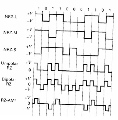

NRZ – Non Return to Zero
Level
NRZ – Non Return to Zero
NRZ – Non Return to Zero
Bipolar Return to Zero
AMI – Alternate Mark Inversion

time division multiplexing
•When each channel has Rb bits/sec bit rate and N such channels are multiplexed, total bit rate = NRb (assuming no added bits)
•Before Multiplexing the bit period = Tb
•After Multiplexing the bit period = Tb/N
•Timing and bit rate would change if you have any added bits

A series of regularly recurring pulses is made to vary in amplitude, duration, shape, or time asa function of the modulating signal

Used to transmit both analog and digital information, such as voice and data.The analog signal is sampled, digitized and encoded into a digital pulse stream.If the signal is already is in digital form, it may be encoded into a digital pulse train.

Initially invented by A.H. Reeves in 1937
Pulse Code Modulation is the representation of a signal by a series of digital pulses firstly by sampling the signal, quantizing it and then encoding it.
The PCM signal itself is a succession of discrete, numerically encoded binary values derived from digitizing the analog signal.
PCM Steps
Sampling
– PAM
– Nyquist sampling rate theorem
Quantizing
– Uniform and non uniform
– A- Law and m- Law
Encoding
– Binary sequences.

Pulse Modulation Examples
Pulse-amplitude modulation (PAM)
Delta modulation (DM)
Pulse-width modulation (PWM)
Pulse-code modulation (PCM)
Pulse-position modulation (PPM)
ADVANTAGES OF PULSE MODULATION
Noise immunity
Inexpensive digital circuitry
Can be time-division multiplexed with other pulse modulated signals
Transmission distance is increased through the use of regenerative repeaters
Digital pulse streams can be stored.
Error detection and correction is easily implemented
DISADVANTAGES OF PULSE MODULATION
Require a much greater bandwidth to transmit and receive than its analog counterpart
Special encoding and decoding techniques may be necessary to increase transmission rates making the pulse stream more difficult to recover.
May require precise synchronization of clocks
between the transmitting and the receiving stations